Age-related nuances in knowledge assessment - Much ado about machine learning
 This is the third post in a series on a paper — “Age-related nuances in knowledge assessment” — we recently published in Intelligence. The first post reflected on how knowledge is organized, the second post dealt with psychometric issues. This post is going to be more mathematical (yes, there will be some formulae) and it will be a cautionary note on the use of machine learning algorithms. Machine learning algorithms have positively influenced research in various scientific disciplines such as astrophysics, genetics, or medicine. Also, subdisciplines in psychology such as personality science (e.g., Stachl et al., 2020) or clinical research (Cearns et al., 2019) are adapting the new statistical tools. However, as pointed out in my research statement, every new method initially bears the risk of applying new techniques without the necessary background knowledge. I mainly blame statistical and methodological courses in psychology studies for this. We really have to teach math, stats, and methods more rigorously in university teaching, especially in structured PhD programs.
Recently, there have been several method-critical papers demonstrating that the implementation of machine learning algorithms in psychology is less than straightforward. Usually1 machine learning algorithms require large samples2, reliable indicators and complete data. Unfortunately, in psychology — in contrast to computer science — we have a different setting. We often rely on small sample sizes, which require special attention to avoid overfitting (Vabalas et al., 2019). Furthermore, typical indicators in psychological research such as questionnaire or test data are subject to measurement errors, which might obscure the true relationship underlying the data (Jacobucci & Grimm, 2020). Finally, to makes things worse, there is often missingness in psychological data sets, either because participants did not answer (irritatingly often referred to as missing by intention) or because not every item was presented to everyone (missing by design). So, this is generally important to keep in mind when using machine learning.
But, what I really wanted to talk about (before I got carried away), are two things in the gc-nuances paper that got stowed away in the Appendix/supplement: First, elastic net is not a magic or alien tool but a little bit more fancy linear regression. Second, given a decent sample size linear regression and its fancier counterpart yield essentially the same results.
A closer look on elastic net regression
To better understand the underlying statistics, I will present some formula, beautifully laid out with ${\KaTeX}$. The loss function of the standard linear regression is denoted by:
$$ \displaystyle\sum_{i=1}^n (y_i - \hat{y} ) ^2 = \Big( {y_i - \displaystyle\sum_{j=1}^p w_j \cdot x_{ij} } \Big)^2 $$
with $x_{ij}$ as the manifest score of a person $i$ on an item $j$ and $w_j$ as weights or regression coefficients. Ridge regression restricts the coefficients by introducing the sum of the squared weights weighted by the shrinkage factor $\lambda$ as a penalty term.
$$ \displaystyle\sum_{i=1}^n \Big( {y_i - \displaystyle\sum_{j=1}^p w_j \cdot x_{ij} } \Big)^2 + \lambda \cdot \displaystyle\sum_{j=1}^p w_{j} ^2 $$
In contrast, least absolute shrinkage and selection operator regression, short LASSO, uses the sum of the absolute weights instead of the squared weights the penalty term, which results in a more parsimonious (and often preferred) procedure (Zou & Hastie, 2005).
$$ \displaystyle\sum_{i=1}^n \Big( {y_i - \displaystyle\sum_{j=1}^p w_j \cdot x_{ij} } \Big)^2 + \lambda \cdot \displaystyle\sum_{j=1}^p |w_{j}| $$
Elastic net regression relies on two regularization parameters—the shrinkage parameter $\lambda$ and the penalty parameter $\alpha$, which balances between ridge and LASSO regression:
$$ \displaystyle\sum_{i=1}^n \Big( {y_i - \displaystyle\sum_{j=1}^p w_j \cdot x_{ij} } \Big)^2 + \lambda \cdot \displaystyle\sum_{j=1}^p (\alpha \cdot w_j^2 + (1 - \alpha) \cdot |w_j|) $$
As one can see from the formula, ridge and LASSO regression are just two special cases of the more general elastic net regression. With the parametrization used here, if $\alpha$ = 1, ridge regression results, whereas LASSO regression is given for $\alpha$ = 0. As a side note: Maybe you start wondering on the last sentence. Wasn’t it the other way around? In the caret documentation it says that if $\alpha$ = 1 you’ll get ridge regression. This inconsistency also bothered me to a certain extend, also because I found both parametrization in The Elements of Statistical Learning. I asked on math stack exchange and got the somehow reassuring answer that there “isn’t an established convention for representing how the elastic net penalty is parameterized”. Anyway, what becomes clear in comparing the formulae, is that elastic net is nothing more than a two-way regularized version of a linear regression.
Comparing linear and elastic net regression
One reason for the use of elastic net is that the regularization — besides cross-validation — serves as statistical countermeasure against overfitting. Overfit describes a statistical phenomenon: A model that was trained on a specific data may be too specific or too complex, so that noise which is always present in real-life data sets is taken for the signal. Accordingly, such a model cannot maintain the accuracy observed in the training sample with a fresh, independent test sample. The difference in prediction accuracy between training and test sample is called overfit. In the online supplement to the paper, we demonstrate with a simulation study that the large sample size is (maybe) the (most) important factor against overfitting.
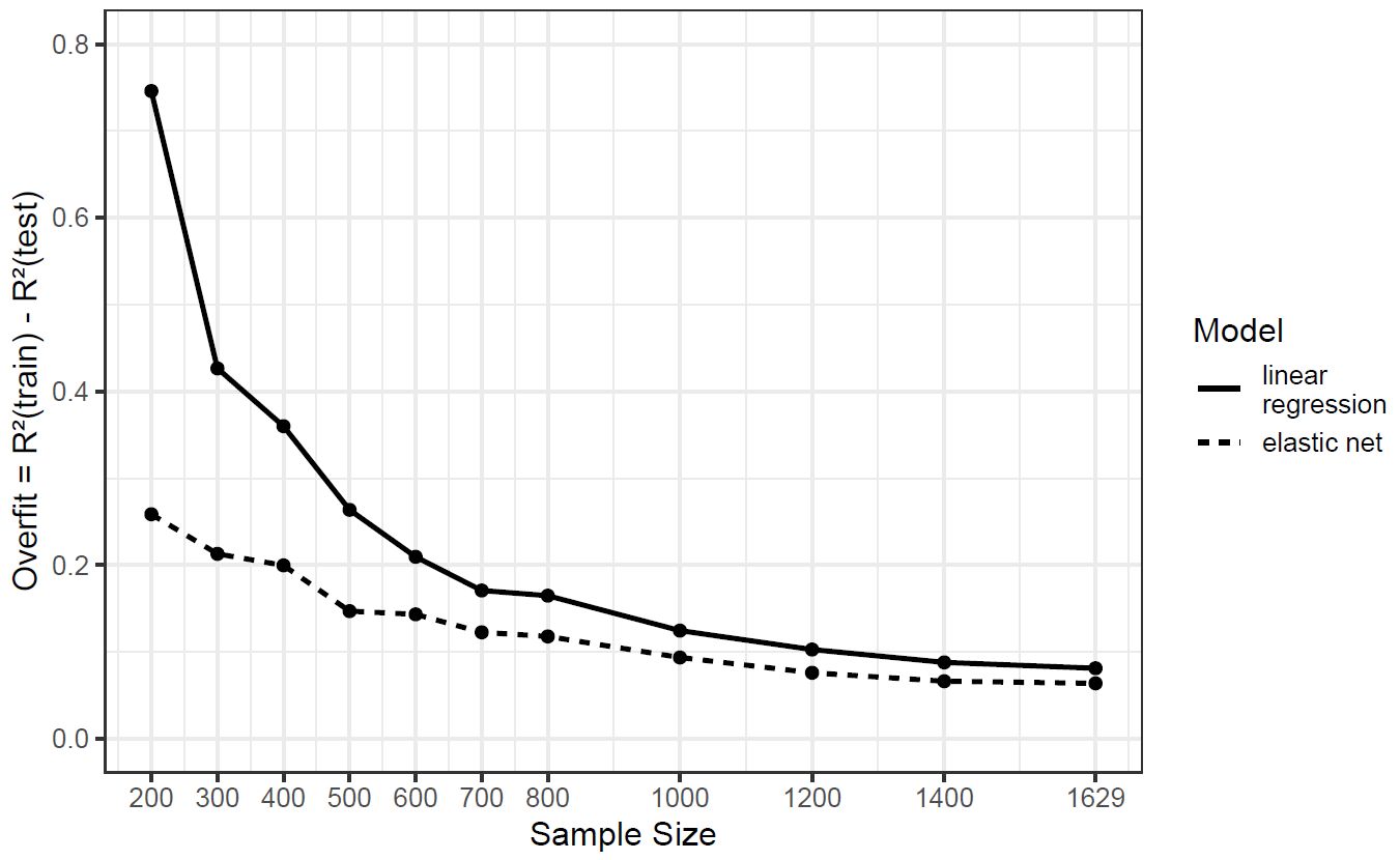
So you might ask, why not simple report the results of the linear regression. As we explain in a footnote we prefer elastic net over linear regressions, out of three reasons: First, because it is the appropriate and versatile method for models with a large number of predictors. Second, because the overfit is still smaller in comparison to linear regression, even in the total sample of more than 1,600 participants. And, third, the elastic models have less predictors, that is, are more parsimonious and thus are easier to interpret.
tl;dr: Elastic net regression is only little bit more fancy than linear regression. Both will yield (almost) identical results with sufficient sample size.
References
- Brandmaier, A. M., von Oertzen, T., McArdle, J. J., & Lindenberger, U. (2013). Structural equation model trees. Psychological Methods, 18(1), 71–86. https://doi.org/10.1037/a0030001
- Cearns, M., Hahn, T., & Baune, B. T. (2019). Recommendations and future directions for supervised machine learning in psychiatry. Translational Psychiatry, 9, Article 271. https://doi.org/10.1038/s41398-019-0607-2
- Jacobucci, R., & Grimm, K. J. (2020). Machine learning and psychological research: The unexplored effect of measurement. Perspectives on Psychological Science, 15(3), 809–816. https://doi.org/10.1177/1745691620902467
- Hastie, T., Tibshirani, H., & Friedman, J. H. (2008). The Elements of Statistical Learning. Springer.
- Stachl, C., Pargent, F., Hilbert, S., Harari, G. M., Schoedel, R., Vaid, S., Gosling, S. D., & Bühner, M. (2020). Personality research and assessment in the era of machine learning. European Journal of Personality. Advance online publication. https://doi.org/10.1002/per.2257
- Vabalas, A., Gowen, E., Poliakoff, E., & Casson, A. J. (2019). Machine learning algorithm validation with a limited sample size. PLOS ONE, 14(11), e0224365. https://doi.org/10.1371/journal.pone.0224365
- Zou, H., & Hastie, T. (2005). Regularization and variable selection via the elastic net. Journal of the Royal Statistical Society, Series B: Statistical Methodology, 67(2), 301–320. https://doi.org/10.1111/j.1467-9868.2005.00503.x
-
Of course, there are special algorithms and techniques to deal with these issues such as semTrees (Brandmaier et al., 2013) for dealing with unreliable indicators. ↩︎
-
As a rule of thumb, one says 1,000 observations. ↩︎